Don Edwards

Department of Statistics, University of South Carolina, Columbia, SC 29208

Abstract. Some basic concepts and strategies for data quality are discussed, specifically: management philosophies; outlier detection for the purpose of elimination of data contamination; keypunch errors; illegal data filter programs; detection of outliers in samples; and detection of outliers and leverage points in simple linear regression.

INTRODUCTION: PREVENTION FIRST

The importance of data quality assurance strategies to long-term ecological research cannot be understated, yet the topic receives surprisingly little attention in the scientific literature. In the short space allotted here, little can be done to comprehensively alleviate this lack of guidance, so one particular issue will be focused on which is highly statistical in nature: the detection of "outliers" in data, as an intermediate step in the elimination of contamination. Before beginning that discussion, though, it must be emphasized that this particular issue is not the most important one to data quality. It is, however, one that has been abused, and one, which this author is qualified to discuss.

Prevention of data contamination is clearly preferable to after-the-fact heroics, but prevention issues are largely management issues. American industry learned the prevention lesson the hard way in the 1960's and 70's, when advancements in quality science in Japan erased American worldwide dominance in the electronics and automobile industries. Ironically, Americans Joseph Juran and W. Edwards Deming, sent to Japan after World War II to help reconstruction, played huge roles in the Japanese coup. As for the relative importance of prevention, no one has expressed it more succinctly than the ever-acidic Deming: "Let's make toast the American industry way - you burn, I'll scrape."

Many management strategies for data quality assurance in scientific settings could be borrowed from industrial quality science. For example, Flournoy and Hearne (1990), in a cancer research center, stress the importance in a multi-user database setting that all users and data contributors have a stake in data quality. In fact, this is also one of Deming's (1986) foundational principles: all company employees, from upper level management (i.e., principal investigators) to line workers (i.e., data entry technicians), must feel a responsibility for, and a pride in, product (i.e., database) quality. Of course, the real challenge lies in inspiring this universal motivation. Along these lines, another surprising Deming principle is that no worker should ever be penalized for poor quality, as poor quality is usually the result of a poorly designed manufacturing (i.e., data collection) process; punishment is unfair and destroys worker-management (i.e., technician-scientist) trust. A successful organizational structure promoted by Deming, which could be adopted immediately for database quality assurance, is the use of "quality circles": these would be regular (e.g., weekly) meetings of scientists, field technicians, systems specialists, and data entry personnel for the purpose of discussing data quality problems and issues. These brief regular meetings build teamwork-attitudes while focusing brain power on data quality issues; participants become constantly aware of quality issues and learn to anticipate problems. Not surprisingly, some of the best ideas come from the lowest-ranking members of the circle!

Incidentally, another of Deming's principles is that everyone, from upper-level management to line workers, should have a basic understanding of natural variability and simple statistical methods for dealing with it. It has been said that one can stop a Japanese at random on the street, and he/she will know the meaning of "standard deviation". In America, asking that question to a random passerby is likely to result in a less desirable outcome!

OUTLIER DETECTION PHILOSOPHY

The term "outlier" is not formally defined. An outlier is simply an unusually extreme value for a variable, given the statistical model in use. What is meant by "unusually extreme" is a matter of opinion, but the operative word here is "unusual"; some extremes are to be expected in any data set. It must also be emphasized, and will be demonstrated, that the "outlier" notion is model-specific: a particular value for a variable might be highly unusual under, say, a linear regression model, but not unusual at all in a model without the regressor. So, outlier detection is part of the process of checking the statistical model assumptions, a process that should be integral to any formal data analysis.

"Elimination of outliers" should not be a goal of data quality assurance. Many ecological phenomena naturally produce extreme values, and to eliminate these values simply because they are extreme is tantamount to pretending that the phenomenon is "well-behaved" when it is not. To mindlessly or automatically do so is to study a phenomenon other than the one of interest. The elimination of data contamination is the appropriate phrasing of this data quality assurance goal. Data contamination occurs when a process or phenomenon other than the one of interest affects a variable's value. If this contamination is undetectable at observation time, it can usually only be detected if it produces an outlying value. Hence, the detection of outliers is an intermediate step in the elimination of contamination. Once the outlier is detected, attempts should be made to determine if some contamination is responsible. This would be a very labor-intensive, expensive step if outliers were not by definition rare. Note also that the investigation of outliers can in some instances be more rewarding than the analysis of the "clean" data: the discovery of penicillin, for example, was the result of a contaminated experiment. If no explanations for a severe outlier can be found, one approach is to formally analyze the data both with and without the outlier(s) and see if conclusions are qualitatively different.

DATA ENTRY ERRORS AND ILLEGAL DATA CHECKS

Sources of contamination due to data entry errors can be eliminated or greatly reduced in several ways. One excellent strategy is to have the data independently keyed by two data entry technicians, and then computer-verified for agreement. This practice is commonplace in professional data entry services, and in some service industries such as the insurance industry (Lepage 1990). Sadly, scientific budgets for data entry are usually inadequate to allow for double-keying of data, though other means of detecting keypunch errors are less effective and probably more expensive since they involve higher-paid personnel.

Illegal data are variable values or combinations of values that are literally impossible for the actual phenomenon of interest. For example, non-integer values for a count variable (e.g., the number of flowers on a plant) or values outside of the interval [0,1] for a proportion variable would be illegal values. Illegal combinations occur when natural relationships among variable values are violated, e.g., if Y₁ is the age of a banded bird in last year's census, and Y₂ is the same bird's age in this year's census, then Y₁ had better be less than Y₂. These kinds of illegal data often occur as data entry errors, but also for other reasons, e.g., misreading of gauges or miswriting of observations in the field or laboratory due to fatigue.

A simple and widely-used technique for detecting these kinds of contamination is an illegal data filter (or "rules," see Henshaw, Bierlmaier, and Hammond, this volume). This is a program which simply checks a laundry-list of variable value constraints on the master data set (or on an update to be added to the master) and creates an output data set including an entry for each violation with identifying information and a message explaining the violation. Table 1 shows the structure of such a program, written in the SAS^TM language (SAS 1990). The filter program can be updated and enhanced to detect new types of illegal data that may have been unanticipated early in the study. A word of caution, however: the operative word here is "illegal". Simply because one has never observed, say, an ozone concentration below a given threshold, and can't imagine it ever happening, does not make such an observation an illegal data point. One of the most famous data QA/QC blunders occurred when NASA computers were programmed to delete satellite observations of ozone concentrations below a specified level, and thus failed to discover the "ozone hole" over the south pole (Stolarski et al. 1986).

Table 1. An illegal-data filter, written in SAS (the data set "All" exists prior to this DATA step, containing the data to be filtered, variable names Y1, Y2, etc., and an observation identifier variable ID).

OUTLIERS IN SAMPLES: GRUBBS' TEST

One of the oldest and most widely used procedures for detecting contamination in samples is Grubbs' test (Grubbs and Beck 1972, ASTM E 1994). By "samples" we mean that, if the data are uncontaminated, we would have several (say, n) independent observations on the variable from the same repeatable, well-defined, stable experimental process. Grubbs' test assumes that the uncontaminated process produces data which follow a Normal (or Gaussian) distribution, and it is very sensitive to that assumption; if the "clean" data are grossly non-Normally distributed, one should not use Grubbs' test. In fact, to this author's knowledge, every formal outlier detection rule / test has the serious drawback that it makes a distributional assumption and is sensitive to that assumption. This is not the case for all statistical procedures that nominally assume Normality; for example, t-tests are typically robust to this assumption.

Grubbs' test is performed as follows: let Y₁<Y₂<...Y_n denote the ordered sample values, and and S the sample mean and standard deviation, respectively. If it is only of interest to detect unusually large outliers, then compare the test statistic

to the appropriate tabled one-sided critical point (Grubbs and Beck 1972, ASTM E 1994), which depends on n and an error rate which we will call a _G. If it is only of interest to detect unusually small outliers, compare the test statistic

to the appropriate one-sided critical point. If either large or small outliers are to be detected, compare the larger of T_n and T₁ to the two-sided critical point.

The probability a _G is in this case a per-sample error rate. So, for example, if a _G is chosen to be .05, then in 5% (1 in twenty) of repeated uncontaminated samples of this size, we would falsely declare a contamination to exist. Users are encouraged to choose a _G thoughtfully, as it has a different meaning than the "a -level" one uses in testing research hypotheses. What fraction of the clean data are you willing to lose, or at the very least investigate, for the sake of detecting possible contamination? Bear in mind that if such contamination is really severe, it would be detected using a smaller a_G, as well. ASTM E (1990) recommends a "low significance level, such as 1%". It should also be noted that Grubbs' test cannot be done at all for n=2, and for n=3 the critical points do not differ for choices of (two-sided) a _G less than .05.

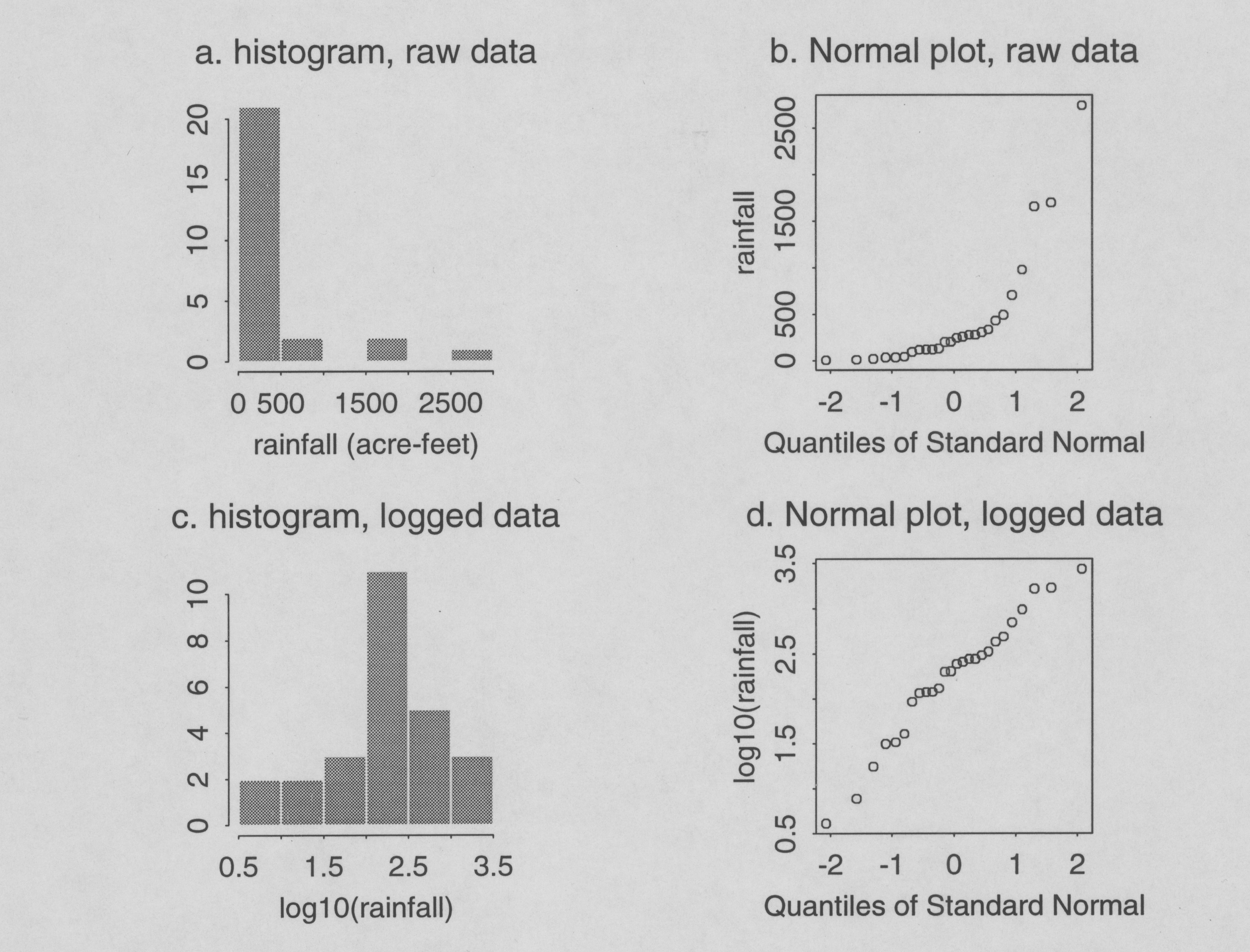
As an example of the (mis-)application of Grubbs' test, consider the seeded-cloud rainfall data of Simpson and colleagues (1975) shown in Table 2. The mean and standard deviation for these data are =442 and S = 651. With n = 26 and a _G=.01, the one-sided critical point for Grubbs' test is 3.029, and the test statistic for detecting large outliers is T₂₆=(2745.6 - 442)/651 = 3.539, hence (if being careless) we would assert contamination.

Table 2. Rainfall in acre-feet from seeded clouds (Simpson et al. 1975).

4.1 7.7 17.5 31.4 32.7 40.6 92.4 115.3 118.3

119.0 129.6 198.6 200.7 242.5 255.0 274.7 274.7 302.8

334.1 430.0 489.1 703.4 978.0 1656.0 1697.8 2745.6

Of course, the assumption that the uncontaminated sample follows a Normal distribution is grossly violated here; Figures 1a and 1b show a histogram and Normal probability plot for the raw data, which clearly show that the sample as a whole follows a severely right-skewed distribution (readers unfamiliar with Normal probability plots can find discussion of them in many modern intermediate statistics texts, e.g., Chambers et al. 1983, Sokal and Rohlf 1981). Figures 1c and 1d show a histogram and Normal plot for the log₁₀-transformed rainfall data. Clearly, these rainfall data are very nearly log-Normally distributed, and there is no evidence of contamination.

Figure 1. Distributional checks of data on rainfall from seeded clouds (Simpson et al. 1975).

OUTLIERS AND INFLUENTIAL POINTS IN REGRESSION

As an example of outlier detection in a multivariable setting, consider the data on 63 species of terrestrial mammals shown in Figure 2, from Allison and Ciccheti (1976). In any study comparing brain weights of animal species, some correction should be made for body weight. One approach to doing this would be to regress brain weight Y on body weight X in some way, and use residuals. Of course, data in a simple linear regression analysis comes in pairs (X₁,Y₁), (X₂,Y₂), ..., (X_n,Y_n). A particular pair can be unusual in at least two ways: Its X-value can be unusually extreme, in which case the pair is referred to as a "leverage point", and/or its Y-value can be unusually extreme relative to the regression line, in which case the point is labeled an outlier. Diagnostics have been defined to measure / detect each of these conditions (Belsley et al. 1980). For example, the leverage of the i^th point is defined to be

i=1,2,...,n, where and are the mean and variance of the regressor. The average value of these h_i values in simple linear regression is 2/n, and the i^th data point is (under some conventions) labeled a "leverage point" if h_i > 4/n. Some authors prefer a more stringent cutoff value, 6/n. At any rate, leverage points are not necessarily bad; they are just more influential in determining the regression line than the other data points. In the regression shown in Figure 2, both the Asian Elephant (h=.1279) and African Elephant (h=.8612) are leverage points.

Figure 2. Brain weights and body weights of 63 species of terrestrial mammals (Allison and Cicchetti 1976).

Outliers in regression can be detected by means of studentized residuals. Several varieties have been defined, but the so-called externally studentized residual is recommended:

where e_i is the i^th ordinary residual (actual Y_i - predicted Y_i) and MSE_(-i) is the error mean square for the regression excluding the i^th pair. Both studentized residuals and leverage points can be obtained (for example) from SAS' PROC REG by requesting their creation in an output data set (SAS 1990).

If the formal assumptions of the regression analysis hold, studentized residuals can be used to test for contamination, since each r_i follows a Student's t-distribution with (n-3) degrees of freedom under the hypothesis of no contamination. Hence, a two-sided test would assert contamination if |r_i| > ta _/2,n-3 , the upper-a /2 critical point from the t distribution with n-3 degrees of freedom. In this case, a is a per-observation error rate, and should again usually be set lower than .05. For example, in a perfectly "clean" data set containing 100 points, we expect 5 studentized residuals to exceed the a =.05 critical value, and 1 to exceed the a =.01 value, purely by accident. No guidelines have been suggested in the literature, but a @ 1/2n appeals to this author. For the data shown in Figure 2, using a = .01, the critical point is t_.005,59 = 2.657 and both of the elephants (r= 12.30 and -11.85) and also Man (r=3.95) flunk the outlier test.

These outlier tests are only valid if the assumptions of the regression hold, however. These assumptions, verbally stated, are:

• The values of the regressor X are known constants (measured with negligible error).
• At any fixed X, the long-run mean of many Y-values, say m(X), is a linear function of X.
• The regression "errors" (the deviations of repeated Y-values at a given X from their long-run mean m(X)) are Normally distributed, with constant variance, and are independent.

In the data of Figure 2, several of these assumptions are either questionable or difficult to assess. Linearity cannot be verified for body weights beyond 1000 kg, since there are so few points at these values. Constant error variance probably doesn't hold, with so many points packed into the lower left hand corner of the plot.

Figure 3. Log₁₀-transformed brain and body weights.

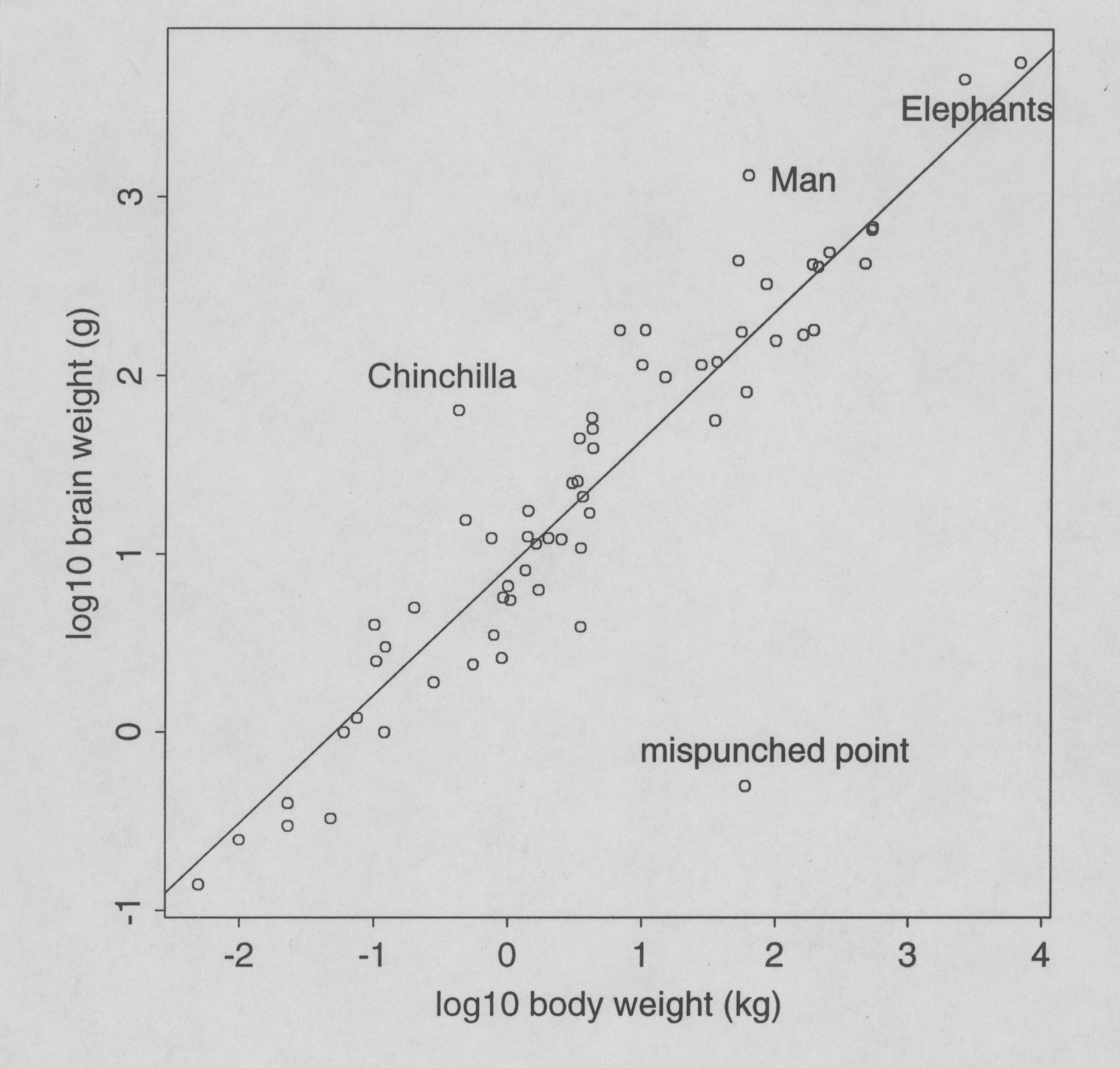
These data vary over several orders of magnitude in both variables, and no analysis of the raw data will distinguish between the lower orders of magnitude. As long as there are elephants in the data, the baboons, lemurs and field mice will all seem equal in size (will all seem to be 0, actually), unless the analysis is done on an order-of-magnitude scale: the log scale. Figure 3 shows a plot of this data in the log scale, i.e. Y*=log₁₀(brain wt) versus X*=log₁₀(body weight). When checked carefully, the formal assumptions of the regression appear to be reasonable, with the possible exception of some points whose Y* values do not fit the pattern (i.e. possible outliers). There are no leverage points now, but the point at lower right in Figure 3, labeled simply as "mispunched point", is a severe outlier since its studentized residual value is r*= -7.56. The point was in fact artificially planted in this data for the purposes of demonstrating a point, but it is also present (but undetectable) in the raw data of Figure 2. It is also undetectable using univariate outlier tests such as Grubbs' test, since both its X and Y-values are separately well within the range of other values found in the data. This point is the promised example of a model-dependent outlier.

Upon removal of the mispunch and reanalysis, two other points in this data set emerge as possible outliers. Man (r* = 2.670) barely signals using a =.01, but the Chinchilla's brain weight (r* = 3.785) is highly unusual given its body weight.

CONCLUSIONS

Some discussion has been offered concerning the prevention and detection of contamination in samples and in regression. Grubbs' test can be adapted to the setting of repeated small samples, as would often be the case in water quality studies, by using a pooled variance estimator over several samples. There are also different versions of the test if one suspects more than one outlier in the sample. Also not discussed is the case of instrument miscalibration, which would result in a possibly large number of "outliers", which are actually shifted variable values, usually by an additive and/or multiplicative constant. Finally, no discussion of modern "robust" statistical methods such as Iteratively Reweighted Least Squares (IRLS) algorithms has been offered (see, e.g., Little 1990). These could, in some cases, be considered to be automatic outlier-detection algorithms; they are potentially very useful, but are still under development. Also, the danger of mindless dependency on automatic detection / elimination algorithms is worrisome.

LITERATURE CITED

Allison, T., and Cicchetti, D.V. 1976. Sleep in mammals: ecological and constitutional correlates. Science 194:732-734.

ASTM E 178-94 1994. Standard practice for dealing with outlying observations. American Society for Testing and Materials, Philadelphia, PA.

Belsley, D.A., E. Kuh, and R.E. Welsch. 1980. Regression diagnostics: identifying influential data and sources of collinearity. John Wiley and Sons, New York, NY.

Chambers, J.M., W.S. Cleveland, B. Kleiner, and P.A. Tukey. 1983. Graphical methods for data analysis. Duxbury Press, Boston, MA.

Deming, W., and D. Edwards. 1986. Out of the crisis. Massachusetts Institute of Technology, Center for Advanced Engineering Study, Cambridge, MA.

Flournoy, N., and L.B. Hearne. 1990. Quality control for a shared multidisciplinary database. Pages 19-23 in G.E. Liepins and V.R.R. Uppuluri, editors. Data quality control: theory and pragmatics. Marcel Dekker, New York, NY.

Grubbs, F.E., and G. Beck. 1972. Extension of sample sizes and percentage points for significance tests of outlying observations. Technometrics 14:847-854.

Lepage, N.J. 1990. Data quality control at United States Fidelity and Guaranty Company. Pages 25-41 in G.E. Liepins and V.R.R. Uppuluri, editors. Data quality control: theory and pragmatics. Marcel Dekker, New York, NY.

Little, R.J. 1990. Editing and imputation of multivariate data: issues and new approaches. Pages 145-166 in G.E. Liepins and V.R.R. Uppuluri, editors. Data quality control: theory and pragmatics. Marcel Dekker, New York, NY.

SAS Institute Inc. 1990. SAS/STAT User's Guide. SAS Institute, Inc., Cary, NC.

Simpson, J., A. Olsen, and J.C. Eden. 1975. A Bayesian analysis of a multiplicative treatment effect in weather modification. Technometrics 17:161-166.

Sokal, R.R., and F.J. Rohlf. 1981. Biometry. W. H. Freeman and Company, New York, NY.

Stolarski, R.S., A.J. Krueger, M.R. Schoeberl, R.D. McPeters, P.A. Newman, and J.C. Alpert. 1986. Nimbus 7 satellite measurements of the springtime Antarctic ozone decrease. Nature 322:808-811.